In part one, we simulated a simple CTMC. Now, let us complicate things a bit. Remember the example problem there:
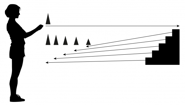
A gas station has a single pump and no space for vehicles to wait (if a vehicle arrives and the pump is not available, it leaves). Vehicles arrive to the gas station following a Poisson process with a rate of  vehicles per minute, of which 75% are cars and 25% are motorcycles. The refuelling time can be modelled with an exponential random variable with mean 8 minutes for cars and 3 minutes for motorcycles, that is, the services rates are
  cars and
  motorcycles per minute respectively (note that, in this context,
  is a rate, not a mean).
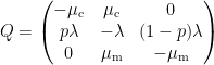
Consider the previous example, but, this time, there is space for one motorcycle to wait while the pump is being used by another vehicle. In other words, cars see a queue size of 0 and motorcycles see a queue size of 1.
The new Markov chain is the following:

where the states car+ and m/c+ represent car + waiting motorcycle and motorcycle + waiting motorcycle respectively.
With  the steady state distribution, the average number of vehicles in the system is given by

lambda <- 3/20
mu <- c(1/8, 1/3)
p <- 0.75
A <- matrix(c(1, 0, 0, mu[1], 0,
1, -(1-p)*lambda-mu[1], mu[1], 0, 0,
1, p*lambda, -lambda, (1-p)*lambda, 0,
1, 0, mu[2], -(1-p)*lambda-mu[2], (1-p)*lambda,
1, 0, 0, mu[2], -mu[2]),
byrow=T, ncol=5)
B <- c(1, 0, 0, 0, 0)
P <- solve(t(A), B)
N_average_theor <- sum(P * c(2, 1, 0, 1, 2)) ; N_average_theor
## [1] 0.6349615
As in the previous post, we can simulate this chain by breaking down the problem into two trajectories (one for each type of vehicle and service rate) and two generators. But in order to disallow cars to stay in the pump’s queue, we need to introduce a little trick in the cars’ seize: the argument amount is a function that returns 1 if the pump is vacant and 2 otherwise. This implies that the car gets rejected, because there is only one position in queue and that seize is requesting two positions. Note also that the environment env must be defined before running the simulation, as it is needed inside the trajectory.
library(simmer)
set.seed(1234)
option.1 <- function(t) {
car <- create_trajectory() %>%
seize("pump", amount=function() {
if (env %>% get_server_count("pump")) 2
else 1
}) %>%
timeout(function() rexp(1, mu[1])) %>%
release("pump", amount=1)
mcycle <- create_trajectory() %>%
seize("pump", amount=1) %>%
timeout(function() rexp(1, mu[2])) %>%
release("pump", amount=1)
env <- simmer() %>%
add_resource("pump", capacity=1, queue_size=1) %>%
add_generator("car", car, function() rexp(1, p*lambda)) %>%
add_generator("mcycle", mcycle, function() rexp(1, (1-p)*lambda))
env %>% run(until=t)
}
The same idea using a branch, with a single generator and a single trajectory.
option.2 <- function(t) {
vehicle <- create_trajectory() %>%
branch(function() sample(c(1, 2), 1, prob=c(p, 1-p)), c(F, F),
create_trajectory("car") %>%
seize("pump", amount=function() {
if (env %>% get_server_count("pump")) 2
else 1
}) %>%
timeout(function() rexp(1, mu[1])) %>%
release("pump", amount=1),
create_trajectory("mcycle") %>%
seize("pump", amount=1) %>%
timeout(function() rexp(1, mu[2])) %>%
release("pump", amount=1))
env <- simmer() %>%
add_resource("pump", capacity=1, queue_size=1) %>%
add_generator("vehicle", vehicle, function() rexp(1, lambda))
env %>% run(until=t)
}
We may also avoid messing up things with branches and subtrajectories. We can decide the type of vehicle and set it as an attribute of the arrival with set_attribute. Then, every activity’s function is able to retrieve those attributes as a named list. Although the branch option is a little bit faster, this one is nicer, because there are no subtrajectories involved.
option.3 <- function(t) {
vehicle <- create_trajectory("car") %>%
set_attribute("vehicle", function() sample(c(1, 2), 1, prob=c(p, 1-p))) %>%
seize("pump", amount=function(attrs) {
if (attrs["vehicle"] == 1 &&
env %>% get_server_count("pump")) 2
else 1
}) %>%
timeout(function(attrs) rexp(1, mu[attrs["vehicle"]])) %>%
release("pump", amount=1)
env <- simmer() %>%
add_resource("pump", capacity=1, queue_size=1) %>%
add_generator("vehicle", vehicle, function() rexp(1, lambda))
env %>% run(until=t)
}
But if performance is a requirement, we can play cleverly with the resource’s capacity and queue size, and with the amounts requested in each seize, in order to model the problem without checking the status of the resource. Think about this:
- A resource with
capacity=3 and queue_size=2.
- A car always tries to seize
amount=3.
- A motorcycle always tries to seize
amount=2.
In these conditions, we have the following possibilities:
- Pump empty.
- One car (3 units) in the server [and optionally one motorcycle (2 units) in the queue].
- One motorcycle (2 units) in the server [and optionally one motorcycle (2 units) in the queue].
Just as expected! So, let’s try:
option.4 <- function(t) {
  vehicle <- create_trajectory() %>%
    branch(function() sample(c(1, 2), 1, prob=c(p, 1-p)), c(F, F),
           create_trajectory("car") %>%
             seize("pump", amount=3) %>%
             timeout(function() rexp(1, mu[1])) %>%
             release("pump", amount=3),
           create_trajectory("mcycle") %>%
             seize("pump", amount=2) %>%
             timeout(function() rexp(1, mu[2])) %>%
             release("pump", amount=2))

  simmer() %>%
    add_resource("pump", capacity=3, queue_size=2) %>%
    add_generator("vehicle", vehicle, function() rexp(1, lambda)) %>%
    run(until=t)
}
We are still wasting time in the branch decision. We can mix this solution above with the option.1 to gain extra performance:
option.5 <- function(t) {
  car <- create_trajectory() %>%
    seize("pump", amount=3) %>%
    timeout(function() rexp(1, mu[1])) %>%
    release("pump", amount=3)

  mcycle <- create_trajectory() %>%
    seize("pump", amount=2) %>%
    timeout(function() rexp(1, mu[2])) %>%
    release("pump", amount=2)

  simmer() %>%
    add_resource("pump", capacity=3, queue_size=2) %>%
    add_generator("car", car, function() rexp(1, p*lambda)) %>%
    add_generator("mcycle", mcycle, function() rexp(1, (1-p)*lambda)) %>%
    run(until=t)
}
Options 1, 2 and 3 are slower, but they give us the correct numbers, because the parameters (capacity, queue size, amounts) in the model remain unchanged compared to the problem. For instance,
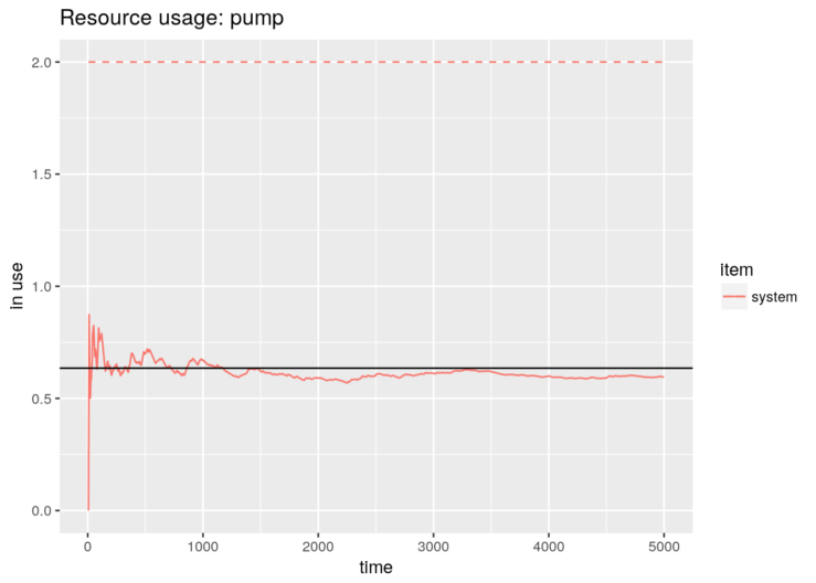
gas.station <- option.1(5000)
library(ggplot2)
graph <- plot_resource_usage(gas.station, "pump", items="system")
graph + geom_hline(yintercept=N_average_theor)
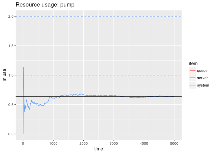
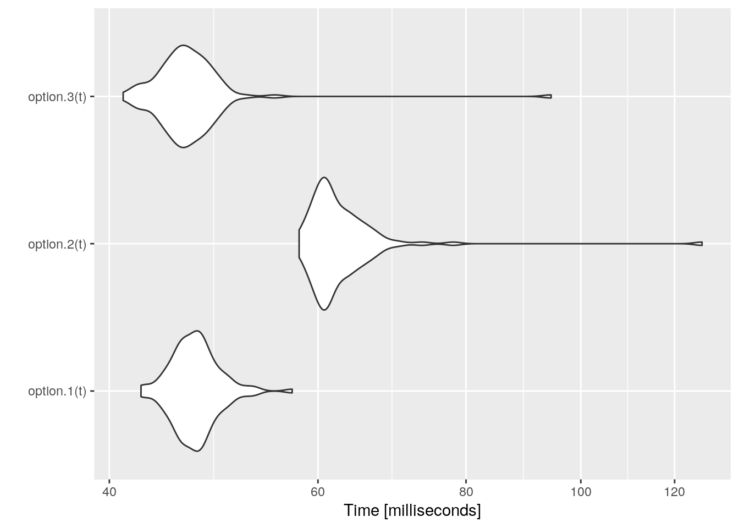
However, it is not the case in options 4 and 5. The parameters of these models have been adulterated to fit our performance purposes. Therefore, we need to extract the RAW data, rescale the numbers and plot them. And, of course, we get the same figure:
gas.station <- option.5(5000)
limits <- data.frame(item = c("queue", "server", "system"), value = c(1, 1, 2))
library(dplyr); library(tidyr)
graph <- gas.station %>% get_mon_resources() %>%
gather(item, value, server, queue, system) %>%
mutate(value = round(value * 2/5),
item = factor(item)) %>%
filter(item %in% "system") %>%
group_by(resource, replication, item) %>%
mutate(mean = c(0, cumsum(head(value, -1) * diff(time))) / time) %>%
ungroup() %>%
ggplot() + aes(x=time, color=item) +
geom_line(aes(y=mean, group=interaction(replication, item))) +
ggtitle("Resource usage: pump") +
ylab("in use") + xlab("time") + expand_limits(y=0) +
geom_hline(aes(yintercept=value, color=item), limits, lty=2)
graph + geom_hline(yintercept=N_average_theor)
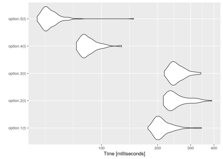
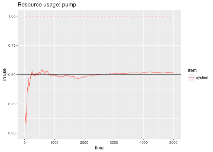
Finally, these are some performance results:
library(microbenchmark)

t <- 1000/lambda
tm <- microbenchmark(option.1(t),
                     option.2(t),
                     option.3(t),
                     option.4(t),
                     option.5(t))
graph <- autoplot(tm)
graph + scale_y_log10(breaks=function(limits) pretty(limits, 5)) +
  ylab("Time [milliseconds]")
## Scale for 'y' is already present. Adding another scale for 'y', which
## will replace the existing scale.
 . The chain is irreducible and recurrent. To theoretically find the steady state distribution, we have to solve the balance equations

 independent columns, so the latter constraint is equivalent to substitute any column by ones and match it to one at the other side of the equation, that is:
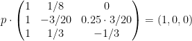

 and
and 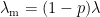 .
.
 ). For instance, people arriving at an ATM at rate
  , waiting their turn in the street and withdrawing money at rate
 ![\begin{aligned} \rho &= \frac{\lambda}{\mu} &&\equiv \mbox{Server utilization} \\ N &= \frac{\rho}{1-\rho} &&\equiv \mbox{Average number of customers in the system (queue + server)} \\ T &= \frac{N}{\lambda} &&\equiv \mbox{Average time in the system (queue + server) [Little's law]} \\ \end{aligned}](https://s0.wp.com/latex.php?latex=%5Cbegin%7Baligned%7D++%5Crho+%26%3D+%5Cfrac%7B%5Clambda%7D%7B%5Cmu%7D+%26%26%5Cequiv+%5Cmbox%7BServer+utilization%7D+%5C%5C++N+%26%3D+%5Cfrac%7B%5Crho%7D%7B1-%5Crho%7D+%26%26%5Cequiv+%5Cmbox%7BAverage+number+of+customers+in+the+system+%28queue+%2B+server%29%7D+%5C%5C++T+%26%3D+%5Cfrac%7BN%7D%7B%5Clambda%7D+%26%26%5Cequiv+%5Cmbox%7BAverage+time+in+the+system+%28queue+%2B+server%29+%5BLittle%27s+law%5D%7D+%5C%5C++%5Cend%7Baligned%7D&bg=ffffff&fg=000&s=0&c=20201002)
 . If that is not true, it means that the system is unstable: there are more arrivals than the server is capable of handling, and the queue will grow indefinitely.
 .
.