errors 0.0.1

In physics, engineering and other disciplines, a single number, a bare quantity, is useless, meaningless. When you measure something, your results will be within the precision of your equipment, and then you need to propagate those errors up to whatever final indirect measure you are interested in. Finally, you need to express it properly. For instance, the elementary charge:

library(errors)

e <- set_errors(1.6021766208e-19, 0.0000000098e-19)
print(e, digits=2, notation="plus-minus")
## (1.6021766208 +/- 0.0000000098)e-19
print(e, digits=2, notation="parenthesis")
## 1.6021766208(98)e-19

Propagation of uncertainty (or propagation of error) is easy, but too labourious. Lately, for various reasons, I have been growing sick of this task, so I decided to write this small package. In a nutshell, the errors package, which is already on CRAN, provides support for painless automatic error propagation in numerical operations and pretty printing.

With errors, you can add errors to your numeric vectors:

x <- 1:10
errors(x) <- 0.1
x
## errors: 0.1 0.1 0.1 0.1 0.1 ...
##  [1]  1  2  3  4  5  6  7  8  9 10
errors(x)
##  [1] 0.1 0.1 0.1 0.1 0.1 0.1 0.1 0.1 0.1 0.1
errors(x) <- seq(0.1, 1, 0.1)
errors(x)
##  [1] 0.1 0.2 0.3 0.4 0.5 0.6 0.7 0.8 0.9 1.0

The set_errors() method is a pipe-friendly version of the above:

(x <- set_errors(1:10, seq(0.1, 1, 0.1)))
## errors: 0.1 0.2 0.3 0.4 0.5 ...
##  [1]  1  2  3  4  5  6  7  8  9 10

Then, you simply work with your quantities without having to worry about errors anymore:

df <- as.data.frame(x)

(df$`3x` <- 3*x)
## errors: 0.3 0.6 0.9 1.2 1.5 ...
##  [1]  3  6  9 12 15 18 21 24 27 30
(df$`x^2` <- x^2)
## errors: 0.2 0.8 1.8 3.2 5 ...
##  [1]   1   4   9  16  25  36  49  64  81 100
(df$`sin(x)` <- sin(x))
## errors: 0.054030230586814 0.0832293673094285 0.296997748980134 0.261457448345445 0.141831092731613 ...
##  [1]  0.8414710  0.9092974  0.1411200 -0.7568025 -0.9589243 -0.2794155
##  [7]  0.6569866  0.9893582  0.4121185 -0.5440211
(df$`cumsum(x)` <- cumsum(x))
## errors: 0.1 0.223606797749979 0.374165738677394 0.547722557505166 0.741619848709566 ...
##  [1]  1  3  6 10 15 21 28 36 45 55

Finally, you probably need to report your data in a consistent way. No problem: just print your table.

df
##         x     3x     x^2  sin(x) cumsum(x)
## 1  1.0(1) 3.0(3)  1.0(2) 0.84(5)    1.0(1)
## 2  2.0(2) 6.0(6)  4.0(8) 0.91(8)    3.0(2)
## 3  3.0(3) 9.0(9)    9(2)  0.1(3)    6.0(4)
## 4  4.0(4)  12(1)   16(3) -0.8(3)   10.0(5)
## 5  5.0(5)  15(2)   25(5) -1.0(1)   15.0(7)
## 6  6.0(6)  18(2)   36(7) -0.3(6)  21.0(10)
## 7  7.0(7)  21(2)  49(10)  0.7(5)     28(1)
## 8  8.0(8)  24(2)  60(10)  1.0(1)     36(1)
## 9  9.0(9)  27(3)  80(20)  0.4(8)     45(2)
## 10  10(1)  30(3) 100(20) -0.5(8)     55(2)

By default, errors uses parenthesis notation (which is more compact) and a single significant digit for errors. If you prefer the plus-minus notation or you need more significant digits, just pass the notation and digits arguments to the print() method, as in the first example, or set them as global options with options(errors.notation="plus-minus", errors.digits=2).

The inner workings of this package have been inspired by Edzer Pebesma and his excellent units package. As a next step, I envision numeric vectors with errors and units for R. Thus, I publicly invite Edzer to collaborate with me in making our packages work together.
Poor man’s parallel con Bash

GNU Parallel es «una herramienta para ejecutar tareas en paralelo usando uno o varias computadoras». Es realmente compleja y versátil, pero muchas veces su uso se reduce a paralelizar un bucle. Algo así, para ejecutar 10 tasks utilizando 4 cores:

[code lang=»bash»]
task() {
echo «running $1…»
sleep $(($1%4))
echo «$1 stopped»
}
export -f task

for i in {1..10}; do
sem -j4 task $i
done
sem –wait
[/code]

Pero si no está disponible o da problemas, y no importa que la salida pueda intercalarse, se puede hacer lo mismo solo con Bash:

[code lang=»bash»]
task() {
echo «running $1…»
sleep $(($1%4))
echo «$1 stopped»
}
pmsem() { ((_i=_i%$1)); ((_i++==0)) && wait -n && ((_i–)); }

for i in {1..10}; do
pmsem 4; task $i &
done
wait
[/code]

simmer 3.6.1

A new patch release of simmer, the Discrete-Event Simulator for R, is on CRAN. Three months have passed since the last release. The last year was a period of intense development (one release per month). Now, the package has reached some level of maturity, so we intend to extend the release cycle.

In this maintenance release, the replacement operators for trajectories ([<-, [[<-) now work as expected. Also, we have removed previously deprecated plotting capabilities, which are covered and extended by the simmer.plot package.

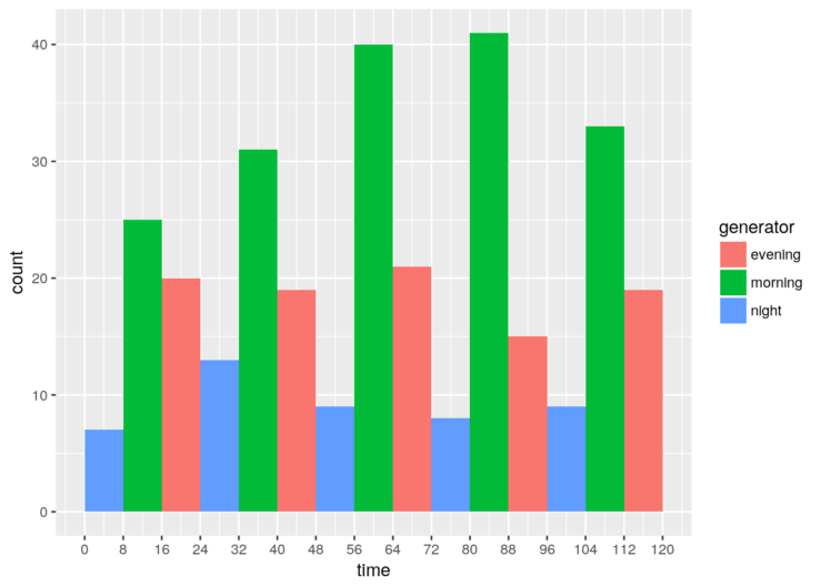
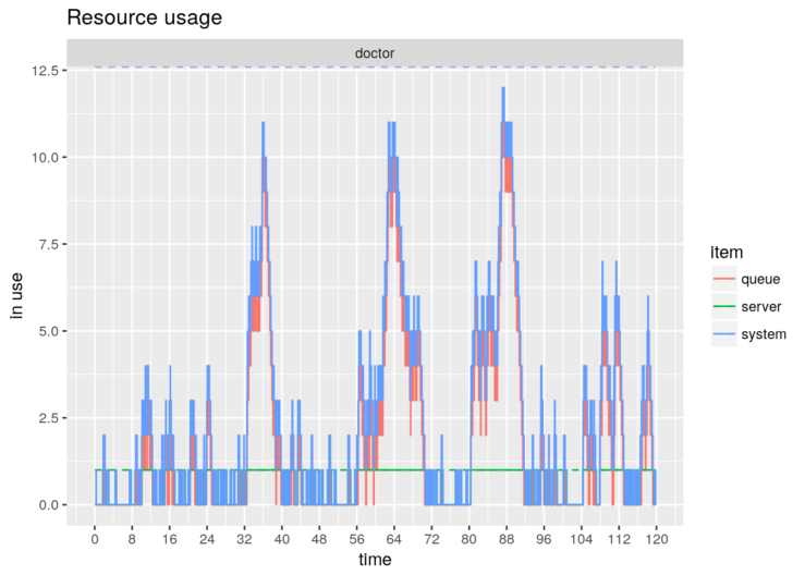
Last but not least, we have extended the from_to() convenience function with a parameter every, which enables the generation of arrivals in cycles. For instance, let us suppose we want to simulate different patient arrival rates in the morning, evening and night:

library(simmer)
library(simmer.plot)
## Loading required package: ggplot2
set.seed(1234)

# units are hours
# visit time between 10 and 20 minutes
patient <- trajectory() %>%
  seize("doctor", 1) %>%
  timeout(function() runif(1, 10/60, 20/60)) %>%
  release("doctor", 1)

morning <- from_to(start_time = 8,
                   stop_time = 16,
                   dist = function() rexp(1, 60/15),
                   arrive = FALSE, 
                   every = 24)

evening <- from_to(start_time = 16,
                   stop_time = 24,
                   dist = function() rexp(1, 60/30),
                   arrive = FALSE, 
                   every = 24)

night   <- from_to(start_time = 0,
                   stop_time = 8,
                   dist = function() rexp(1, 60/60),
                   arrive = FALSE, 
                   every = 24)

env <- simmer() %>%
  add_resource("doctor", 1) %>%
  add_generator("morning", patient, morning) %>%
  add_generator("evening", patient, evening) %>%
  add_generator("night",   patient, night) %>%
  run(24 * 5) # simulate 5 days

breaks <- c(0, cumsum(rep(8, 3 * 5)))

env %>%
  get_mon_arrivals() %>%
  dplyr::mutate(generator = factor(gsub("\\d", "", name))) %>%
  ggplot(aes(start_time, fill=generator)) + xlab("time") +
  stat_bin(breaks = breaks) +
  scale_x_continuous(breaks = breaks)

plot(env, what="resources", metric="usage", "doctor", steps=TRUE) +
  scale_x_continuous(breaks = breaks)

Minor changes and fixes:

  • Recycle logical indexes when subsetting (2526e75).
  • Implement replacement operators, [<- and [[<- (#88).
  • Provide rep() S3 method for trajectories (7fa515e).
  • Remove plotting functions (bb9656b), deprecated since v3.6.0. The new simmer.plot package (on CRAN) already covers these features among others.
  • Don’t evaluate vignette chunks if Suggests are not installed (e40e5b6).
  • Rewrite DESCRIPTION (3f26516).
  • Add an every parameter to the from_to() convenience function (9d68887).

Suggests and Vignettes

Dirk Eddelbuettel quite rightly reminded us the other day that Suggests is not Depends. I am sorry to say that I am one of those who are using Suggests… “casually”. Mea culpa. I must say that this is restricted to vignettes: there are no tests nor examples using suggested packages. But I am not checking if my suggested packages are available at all, which is definitely wrong. And I understand that it must be frustrating to run reverse dependencies on a package as popular as Rcpp when the rest of us are using Suggests so… casually. So I was definitely determined to solve this, and I finally managed to find a very simple solution that may be helpful to other maintainers.

Our simmer package has seven vignettes. Two of them are very introductory and do not use any external package. But as you try to demonstrate more advanced features and use cases, you start needing some other tools; and their use could be intensive, so that checking suggested packages for every call or every code chunk might not scale. However, I realised that the important thing for those advanced vignettes is just to make the story they tell available to your users, and anyway they are always built and available online on CRAN. Therefore, I decided to add the following at the beginning of each vignette:

required <- c("pkg1", "pkg2", "pkgn")

if (!all(sapply(required, requireNamespace, quietly = TRUE)))
  knitr::opts_chunk$set(eval = FALSE)

Problem solved. Yes, I know, I am still taking knitr for granted. But given that it has its own entry (VignetteBuilder) in the DESCRIPTION, I think this is fair enough. I only hope that Dirk will unblacklist simmer after our next release. ;-)

Periodismo de datos sin datos

(Esta anotación se publica simultáneamente en Naukas)

Me encuentro en Twitter con el siguiente gráfico despropósito de CBS News:

donde se hace referencia al porcentaje de estadounidenses que dice haber probado la marihuana. Evidentemente, los porcentajes no suman 100 % porque se refieren a una misma población en tres instantes temporales diferentes. Evidentemente, digo, si uno lee todo el texto y se para a digerir lo que está viendo, por lo que mostrar una gráfica pierde toda su razón de ser.

Gráficas horribles como esta constituyen, desafortunadamente, la tónica generalizada en los medios de comunicación, con mención especial para la televisión. Pero esta en concreto me ha llamado especialmente la atención porque, paradójicamente, la torpeza en la representación esconde un despropósito mucho mayor que tiene que ver con los datos (o su ausencia, más bien).

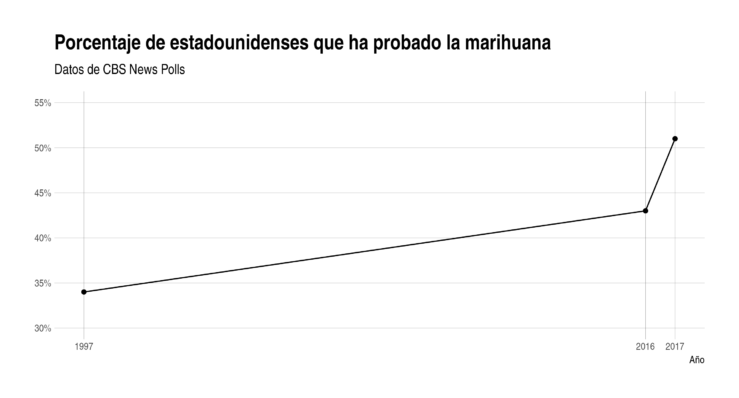
Desconozco si CBSN quería decirnos simplemente que mucha gente apoya la legalización de la marihuana, como reza el titular. Si es así, no entiendo qué tiene que ver el porcentaje de gente que la ha probado y, en todo caso, el dato de hoy en día sería más que suficiente. Por el contrario, la elección de la pregunta y los datos históricos sugieren más bien que el número de fumetas se ha disparado peligrosamente (crecimiento de 9 puntos en 19 años y ¡8 puntos en el último año!). Pero independientemente de su intención, la representación de una serie temporal debe hacerse de la siguiente manera:

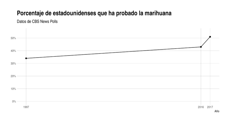
Además, cuando hablamos de porcentajes, lo ideal es comprimir el eje hasta mostrar la referencia del 0 %:

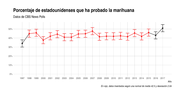
Desatinos aparte, se agradece que CBSN especifique el margen de error, que es del +/- 4 % (con un nivel de confianza del 95 %, asumo, por lo que podemos inferir que el número de encuestados se sitúa entre 500 y 1000 personas). Una última mejora, por tanto, pasaría por añadir dicho margen de error:

Ahora tenemos una buena gráfica, pero el problema de fondo persiste: estamos haciendo periodismo de datos sin datos. ¿Qué hay entre 1997 y 2016? No lo sabemos (y no sabemos si lo saben), y por tanto no hay manera de interpretar el aparente crecimiento del último año. Podemos hacer, no obstante, el ejercicio de inventarnos unos cuantos datos, aunque sea de manera chabacana, y ver cómo podría cambiar el cuento:

Simplemente he cogido la media de los datos de 1997 y hoy y he generado valores según una normal de desviación adecuada al margen de error. Como resultado, el efecto de crecimiento acelerado desaparece. En definitiva, parece claro que ha habido un incremento desde el año 1997, pero poco o nada podemos decir del incremento del último año.